In this introductory 101 article, we’ll cover the basics of how to ingest CSV data into TileDB so that it can be accessed as pandas dataframes. I'll cover slicing and querying via SQL, with the goal of keeping everything self-contained to help folks get up to speed.

Setup

This tutorial can run end-to-end locally on your own machine using the TileDB open-source library, called TileDB Embedded. I will also use the TileDB Python API, noting that TileDB offers a large variety of other APIs as well. You will need to download this small CSV (4 KB) based on the NYC TLC trip record data for yellow taxis. I recommend activating a fresh conda environment and then running:

conda install -c conda-forge tiledb-py libtiledb-sql-py pyarrow pandas sqlalchemy

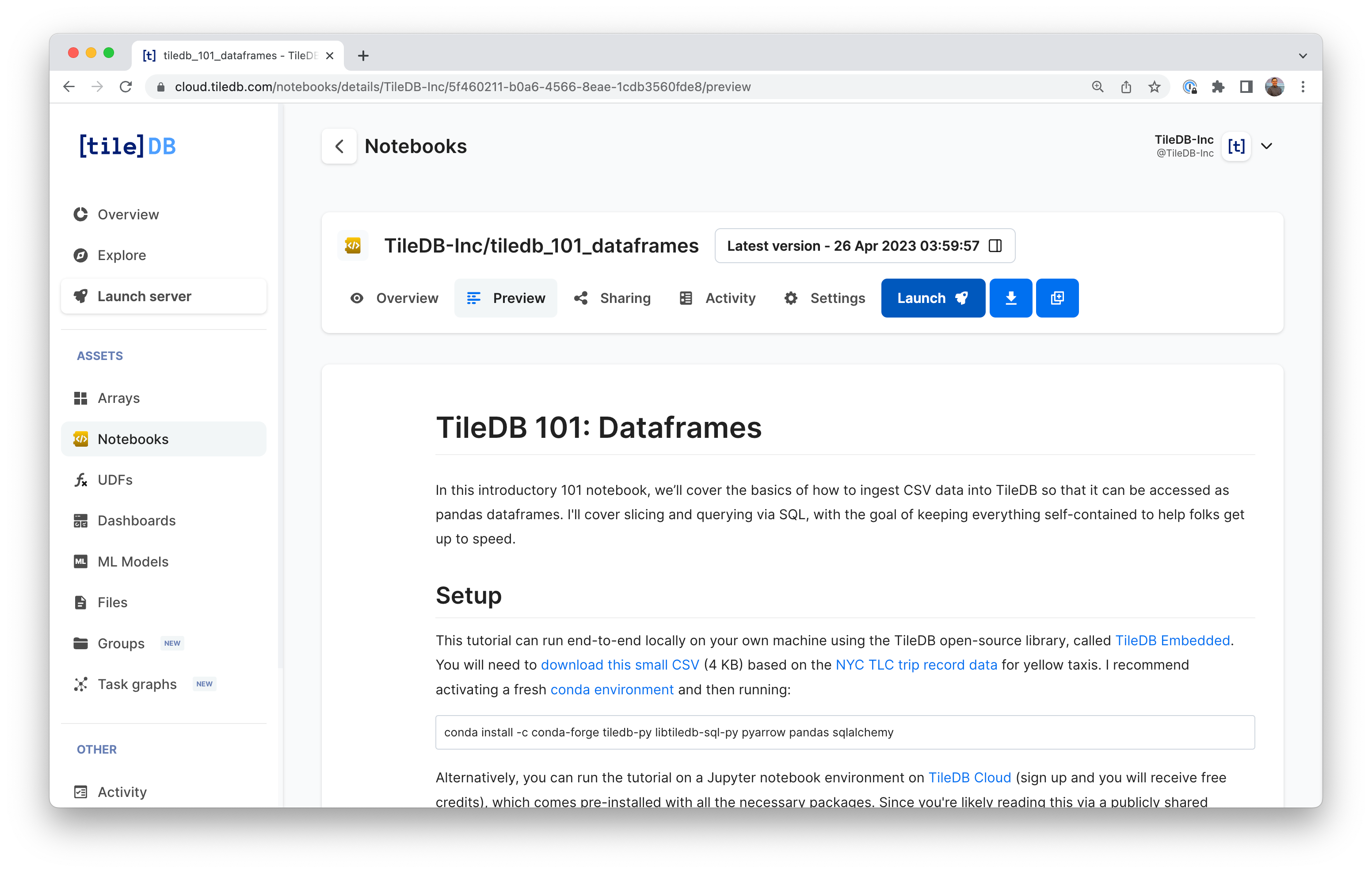
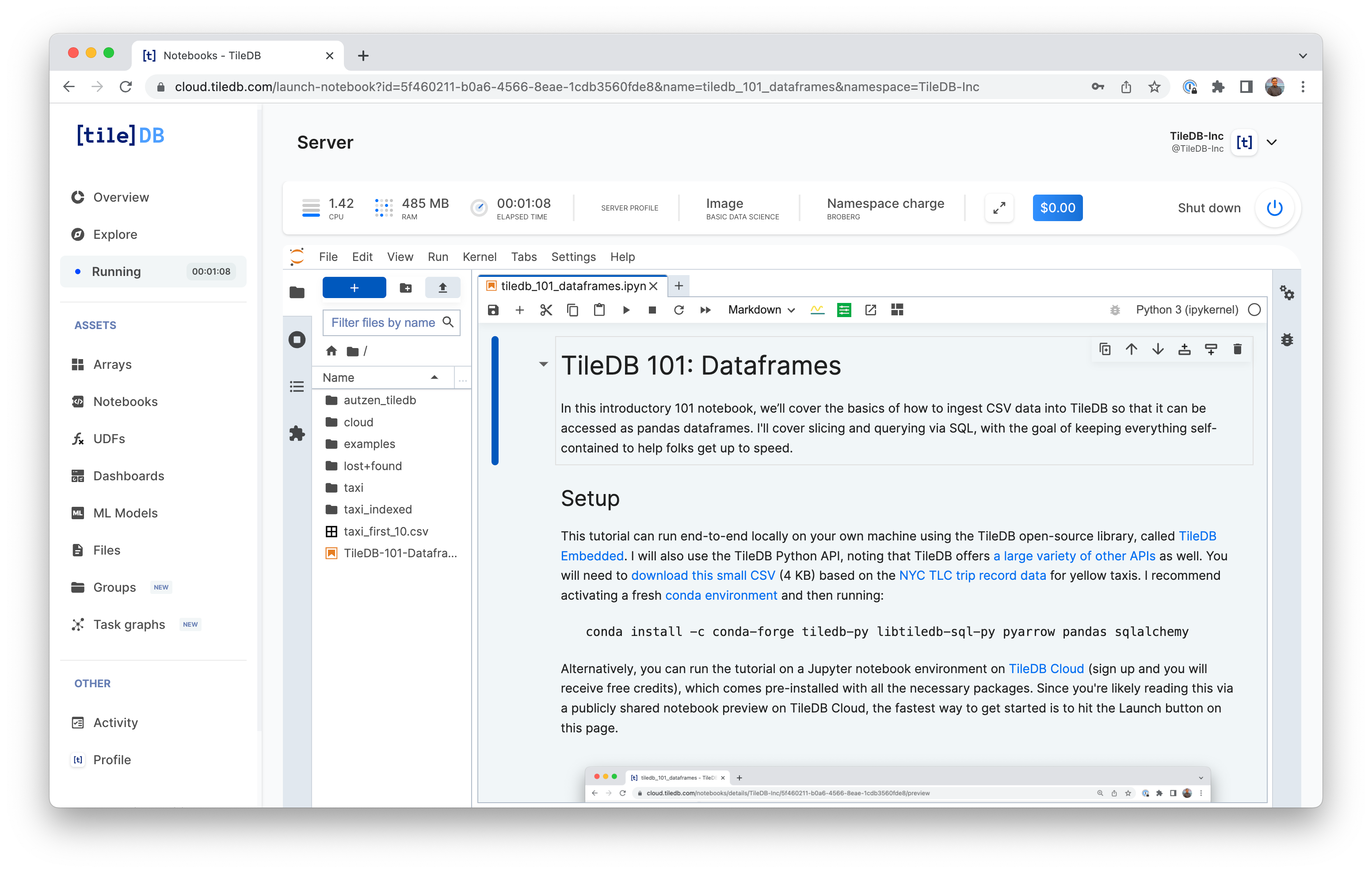
Alternatively, you can run the tutorial on a Jupyter notebook environment on TileDB Cloud (sign up and you will receive free credits), which comes pre-installed with all the necessary packages (full notebook here). To launch a notebook server on TileDB Cloud, hit the Launch button on the notebook's preview page:

From a Python Jupyter notebook, run your import statements:

import tiledb
import numpy as np

If you're using TileDB Cloud like I am, then you can upload the CSV to your notebook user's home directory using the JupyterLab UI:

Basic ingestion

To start, I'll use my CSV of 10 taxi rides and TileDB’s from_csv() ingestor method to quickly import data and start working with it in pandas. Since I already know there are dates in this dataset, an additional parameter instructs TileDB to parse certain columns as datetime objects.

tiledb.from_csv("taxi", "taxi_first_10.csv",  
                parse_dates=['tpep_dropoff_datetime', 'tpep_pickup_datetime'])

A = tiledb.open("taxi")
print(A.schema)

When I check the schema, here’s what I get:

ArraySchema(
  domain=Domain(*[
    Dim(name='__tiledb_rows', domain=(0, 9), tile=9, dtype='uint64', filters=FilterList([ZstdFilter(level=-1), ])),
  ]),
  attrs=[
    Attr(name='VendorID', dtype='int64', var=False, nullable=False, filters=FilterList([ZstdFilter(level=-1), ])),
    Attr(name='tpep_pickup_datetime', dtype='datetime64[ns]', var=False, nullable=False, filters=FilterList([ZstdFilter(level=-1), ])),
    Attr(name='tpep_dropoff_datetime', dtype='datetime64[ns]', var=False, nullable=False, filters=FilterList([ZstdFilter(level=-1), ])),
    Attr(name='passenger_count', dtype='int64', var=False, nullable=False, filters=FilterList([ZstdFilter(level=-1), ])),
    Attr(name='trip_distance', dtype='float64', var=False, nullable=False, filters=FilterList([ZstdFilter(level=-1), ])),
    Attr(name='RatecodeID', dtype='int64', var=False, nullable=False, filters=FilterList([ZstdFilter(level=-1), ])),
    Attr(name='store_and_fwd_flag', dtype='<U0', var=True, nullable=False, filters=FilterList([ZstdFilter(level=-1), ])),
    Attr(name='PULocationID', dtype='int64', var=False, nullable=False, filters=FilterList([ZstdFilter(level=-1), ])),
    Attr(name='DOLocationID', dtype='int64', var=False, nullable=False, filters=FilterList([ZstdFilter(level=-1), ])),
    Attr(name='payment_type', dtype='int64', var=False, nullable=False, filters=FilterList([ZstdFilter(level=-1), ])),
    Attr(name='fare_amount', dtype='float64', var=False, nullable=False, filters=FilterList([ZstdFilter(level=-1), ])),
    Attr(name='extra', dtype='float64', var=False, nullable=False, filters=FilterList([ZstdFilter(level=-1), ])),
    Attr(name='mta_tax', dtype='float64', var=False, nullable=False, filters=FilterList([ZstdFilter(level=-1), ])),
    Attr(name='tip_amount', dtype='float64', var=False, nullable=False, filters=FilterList([ZstdFilter(level=-1), ])),
    Attr(name='tolls_amount', dtype='int64', var=False, nullable=False, filters=FilterList([ZstdFilter(level=-1), ])),
    Attr(name='improvement_surcharge', dtype='float64', var=False, nullable=False, filters=FilterList([ZstdFilter(level=-1), ])),
    Attr(name='total_amount', dtype='float64', var=False, nullable=False, filters=FilterList([ZstdFilter(level=-1), ])),
    Attr(name='congestion_surcharge', dtype='float64', var=False, nullable=False, filters=FilterList([ZstdFilter(level=-1), ])),
  ],
  cell_order='row-major',
  tile_order='row-major',
  capacity=10000,
  sparse=False,
)

Since this is a 101 blog, I'm going to use the default settings. In future articles, we'll cover additional configurations to control compression filters, on-disk layouts, and more.

All data in TileDB are represented as multi-dimensional arrays, and this basic CSV ingestion created a 1D dense array, whose dimension name is __tiledb_rows and with domain [0,9] which indicated that there are 10 rows. Every one of the 18 columns in the CSV is modeled as an array attribute, which (by default) will be compressed with zstd (TileDB is a columnar format like Parquet).

The important thing to know at this point is that, the way I created this array, I can do two operations very fast:

• I can efficiently slice any range of rows (e.g., [3-5]).
• I can efficiently select any subset of attributes (e.g., only VendorID and passenger_count).

Basic slicing

We can slice all of the data into a pandas dataframe using TileDB's df[] operator like so:

A.df[:] # Equivalent to: A.df[0:9]

You should get the pandas pretty-printed output, with the row index in the left-most column:

To slice a subset of rows, simply pass the desired range in the df operator:

A.df[3:5]

When using TileDB's df operator, note that [3:5] is open on the right side, returning rows 3, 4 and 5. This is different from numpy arrays, where ranges are closed on the right side, and the same [3:5] slice would return only rows 3 and 4.

You can subselect on the attributes using query as follows:

A.query(attrs=('tip_amount', 'trip_distance')).df[:]

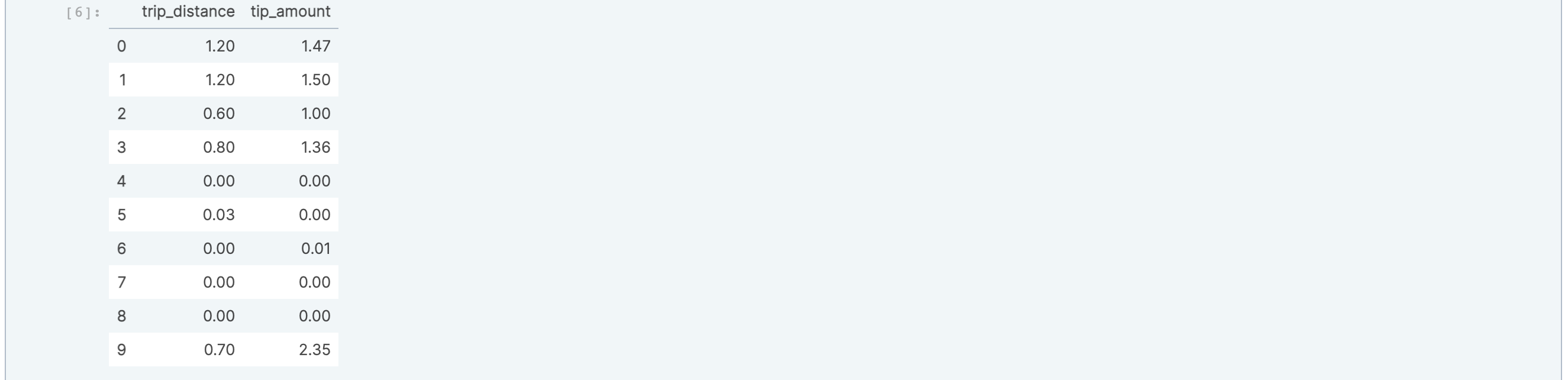
It's a best practice to close the array when you're done working with it.

A.close()

Multi-column indexing

The previous CSV ingestion allowed for fast row slicing. You can also ingest tabular data using a multi-column index, which allows fast range slicing on any subset of columns. TileDB supports this via ingestion into ND sparse arrays, where the dimensions are the columns you wish to slice fast on.

Let's revisit the from_csv() ingestor to ingest the CSV into a 2-dimensional array. First, we need to declare which columns from our CSV will become the indexes of our dataframe, say tpep_dropoff_datetime and fare_amount. These columns are declared as TileDB array dimensions. In the TileDB view of the world, this will transform the table into a 2D sparse array under the hood, where slicing on these two columns will become rapid.

tiledb.from_csv("taxi_indexed", "taxi_first_10.csv", 
                index_col=['tpep_dropoff_datetime', 'fare_amount'], 
                parse_dates=['tpep_dropoff_datetime', 'tpep_pickup_datetime'])

Note above that we use index_col to specify the two columns to be indexed. Next, let's inspect the array's schema:

B = tiledb.open("taxi_indexed")
print(B.schema)

This produces the following output:

ArraySchema(
  domain=Domain(*[
    Dim(name='tpep_dropoff_datetime', domain=(numpy.datetime64('2019-12-18T15:28:59.000000000'), numpy.datetime64('2020-01-01T01:00:14.000000000')), tile=numpy.timedelta64(1000,'ns'), dtype='datetime64[ns]', filters=FilterList([ZstdFilter(level=-1), ])),
    Dim(name='fare_amount', domain=(0.01, 8.0), tile=8.0, dtype='float64', filters=FilterList([ZstdFilter(level=-1), ])),
  ]),
  attrs=[
    Attr(name='VendorID', dtype='int64', var=False, nullable=False, filters=FilterList([ZstdFilter(level=-1), ])),
    Attr(name='tpep_pickup_datetime', dtype='datetime64[ns]', var=False, nullable=False, filters=FilterList([ZstdFilter(level=-1), ])),
    Attr(name='passenger_count', dtype='int64', var=False, nullable=False, filters=FilterList([ZstdFilter(level=-1), ])),
    Attr(name='trip_distance', dtype='float64', var=False, nullable=False, filters=FilterList([ZstdFilter(level=-1), ])),
    Attr(name='RatecodeID', dtype='int64', var=False, nullable=False, filters=FilterList([ZstdFilter(level=-1), ])),
    Attr(name='store_and_fwd_flag', dtype='<U0', var=True, nullable=False, filters=FilterList([ZstdFilter(level=-1), ])),
    Attr(name='PULocationID', dtype='int64', var=False, nullable=False, filters=FilterList([ZstdFilter(level=-1), ])),
    Attr(name='DOLocationID', dtype='int64', var=False, nullable=False, filters=FilterList([ZstdFilter(level=-1), ])),
    Attr(name='payment_type', dtype='int64', var=False, nullable=False, filters=FilterList([ZstdFilter(level=-1), ])),
    Attr(name='extra', dtype='float64', var=False, nullable=False, filters=FilterList([ZstdFilter(level=-1), ])),
    Attr(name='mta_tax', dtype='float64', var=False, nullable=False, filters=FilterList([ZstdFilter(level=-1), ])),
    Attr(name='tip_amount', dtype='float64', var=False, nullable=False, filters=FilterList([ZstdFilter(level=-1), ])),
    Attr(name='tolls_amount', dtype='int64', var=False, nullable=False, filters=FilterList([ZstdFilter(level=-1), ])),
    Attr(name='improvement_surcharge', dtype='float64', var=False, nullable=False, filters=FilterList([ZstdFilter(level=-1), ])),
    Attr(name='total_amount', dtype='float64', var=False, nullable=False, filters=FilterList([ZstdFilter(level=-1), ])),
    Attr(name='congestion_surcharge', dtype='float64', var=False, nullable=False, filters=FilterList([ZstdFilter(level=-1), ])),
  ],
  cell_order='row-major',
  tile_order='row-major',
  capacity=10000,
  sparse=True,
  allows_duplicates=True,
)

Note that this is a 2D sparse array, consisting of a datetime dimension and a float dimension, along with 16 attributes. That is, all 18 CSV columns were ingested, but two of them are indexed (the dimensions).

Slicing in two dimensions

We can again slice the whole array into a pandas dataframe using TileDB's df operator.

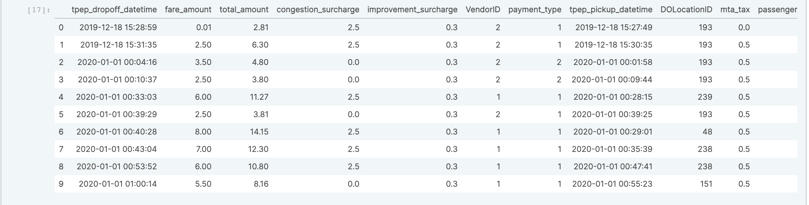
B.df[:] # Equivalent to B.df[:, :]

This returns the following, with the dimensions appearing in the left-most columns as pandas indexes:

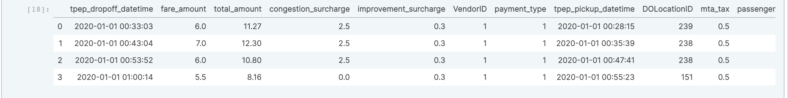
We can slice on the first dimension. Here, we look for rides that dropped off within the first 30 minutes of 2020:

ts1 = np.datetime64('2020-01-01T00:00:00')
ts2 = np.datetime64('2020-01-01T00:30:00')
B.df[ts1:ts2]

We can also slice multiple dimensions. First, slice by the entire first dimension, and then enter the range for the second dimension to return fares between $5 and $7. Again, note that slicing using the df operator is inclusive.

B.df[:, 5.0:7.0]

Of course, you can slice ranges across both dimensions too:

B.df[ts1:ts2, 2.0:3.0]

Querying on attributes

In addition to querying on indexed columns (the dimensions), TileDB allows you to apply filter conditions on attributes as well. Querying on attributes will not be as fast as on dimensions; however, TileDB has a lot of internal engineering magic to make such queries super efficient.

You can apply filter conditions on attributes as follows:

B.query(cond="tip_amount > 0.01 and tip_amount < 2.00", attrs=('tip_amount', 'trip_distance')).df[:]

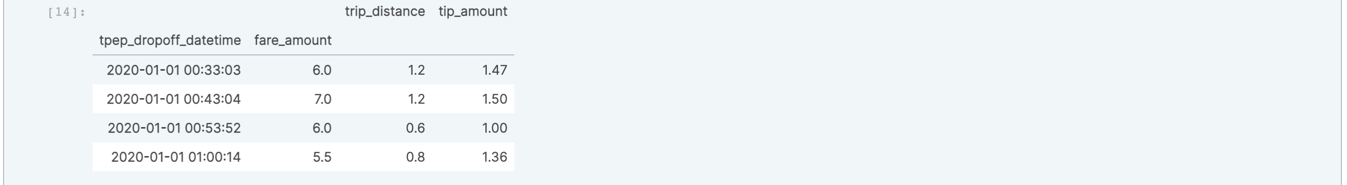
SQL

TileDB provides an integration with MariaDB for embedded (i.e., serverless) SQL. Follow the installation instructions, and import the following packages:

import tiledb.sql
import pandas as pd

If you get a warning message, you can safely ignore mysql error number 2000; it is an artifact of the way TileDB embeds MariaDB as a library (MariaDB is looking for tables that do not exist since there is no server running).

From here, create a connection object and use pandas's read_sql method:

db = tiledb.sql.connect(init_command="SET GLOBAL time_zone='+00:00'")
pd.read_sql(sql="select * from `taxi_indexed`", con=db)

It's worth noting here that MariaDB will default to your system timezone, but in order to keep the results consistent, I'm using a mysql command-line option to set the timezone to UTC when I create the connection. This should produce the same output as B.df[:] above:

We can write the equivalent SQL to one of our fare queries above:

pd.read_sql(sql="select * from `taxi_indexed` where `fare_amount` >= 5.0 and `fare_amount` <= 7.0", con=db)

Of course, you also have access to SQL functions to aggregate columns like tip_amount:

pd.read_sql(sql="SELECT AVG(tip_amount) FROM `taxi_indexed`", con=db)

I got $0.769 as an average tip, but this is a super-small sample, and the trips are short.

See you next time

That's it for TileDB 101: Dataframes! You can preview and download the notebook from TileDB Cloud. This version includes a few extras to make it easier to reference data stored in your TileDB Cloud user directory.

We'd love to hear what you think of this article. Join our Slack community, or let us know on Twitter and LinkedIn. Look out for future articles in our 101 series on TileDB. Until next time!