Why Arrays as a Universal Data Model

These are exciting times for anyone working on data problems, as the data industry is as hot and as hyped as ever. Numerous databases, data warehouses, data lakes, lakehouses, feature stores, metadata stores, file managers, etc. have been hitting the market in the past few years. I have spent my entire career in data management, but going against the market trend, I have always been absolutely baffled that we keep on creating a new data system for every different data type and application. During my time at Intel Labs and MIT between 2014–2017 where I worked as a database researcher, I asked myself a simple question: instead of building a new data system every time our data needs change, can we build a single database that can store, govern, and process all data — tables, images, video, genomics, LiDAR, features, metadata, flat files and any other data type that may pop up in the future.

This question was born from the simple observation that all database systems (and variations) share significant similarities, including laying data out on the storage medium of choice, and fetching it for processing based on certain query workloads. Therefore, to answer the above question, I had to ask a slightly different one: is there a data model that can efficiently capture all data from all applications? Because if such a universal data model exists, it can serve as the foundation for building a universal database with all the subsystems common to all databases (query planner, executor, authenticator, transaction manager, APIs, etc.). In this blog post I argue that such a model does exist, and it is based on multi-dimensional arrays.

Before elaborating on why arrays are universal, I need to answer yet another question: why should you care about a universal data model and a universal database? Here are a few important reasons:

• Data diversity. You may think that it’s all about tabular data for which a traditional data warehouse (or data lake, or lakehouse) can do the trick, but in reality organizations possess a ton of other very valuable data, such as images, video, audio, genomics, point clouds, flat files and many more. And they wish to perform a variety of operations on these data collections, from analytics, to data science and machine learning.
• Vendor optimization. In order to be able to manage their diverse data, organizations resort to either buying numerous different data systems, e.g., a data warehouse, plus an ML platform, plus a metadata store, plus a file manager. That costs money and time; money because some of the vendors have overlapping functionality that you pay twice for (e.g., authentication, access control, etc), and time because teams have to learn to operate numerous different systems, and wrangle data when they need to gain insights by combining disparate data sources.
• Holistic governance. Even if organizations are happy with their numerous vendors, each different data system has its own access controls and logging capabilities. Therefore, if an organization needs to enforce centralized governance over all its data, it needs to build it in-house. That costs more money and time.

Even if I have already managed to convince you of the importance of a universal database, I need to make one last vital remark. A universal database is unusable if it does not offer excellent performance for all the data types it is serving. In other words, a universal database must be performing as efficiently as the purpose-built ones, otherwise there will be a lot of skepticism on adopting it. And this is where the difficulty of universal databases lies and why no one is building such a system today (well, almost no one).

In this blog post I show that multi-dimensional arrays are the right bet not only for their universality, but also for their performance. In full disclosure, I am the founder and CEO of TileDB, a company that is building a universal database with multi-dimensional arrays as first class citizens. I will include a lot of the critical decisions we took at TileDB when designing the array data model, an efficient on-disk format and a powerful storage engine to support it. My goal is to emphasize the generic array principles, hoping that this article can serve as a small step towards shifting from purpose-built data systems to developing more universal databases.

Take a deep breath, we are about to take a technical dive!

The rest of the blog post is for you if:

• You work with a single data type (tables, genomics, LiDAR, imaging, etc) and potentially use a special-purpose data system, but you’d like to deeply understand how multi-dimensional arrays could offer an elegant and more performant solution for your use case.
• You work with diverse data from many sources using modern native tools, and want to understand the technical design choices which make multi-dimensional arrays capable and adaptable to any dataset or workload through a common format, engine and interface.
• It is important for you to understand the foundations of the tools you explore to use and compare, and need to be certain that they are well-designed to meet your requirements now and in the future.

The array data model

The basic array model we follow at TileDB is depicted below. We make an important distinction between a dense and a sparse array. A dense array can have any number of dimensions. Each dimension must have a domain with integer values, and all dimensions have the same data type. An array element is defined by a unique set of dimension coordinates and it is called a cell. In a dense array, all cells must store a value. A logical cell can store more than one value of potentially different types (which can be integers, floats, strings, etc). An attribute defines a collection of values that have the same type across all cells. A dense array may be associated with a set of arbitrary key-value pairs, called array metadata.

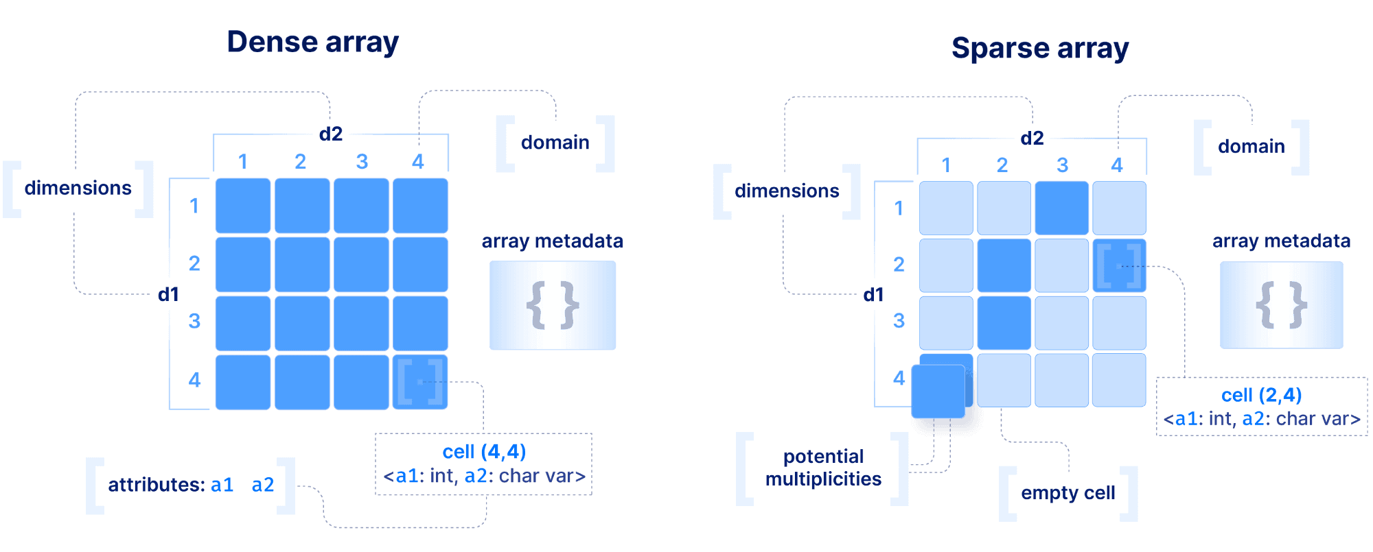
A sparse array is very similar to a dense array, but it has three important differences:

1. Cells in a sparse array can be empty.
2. The dimensions can have heterogeneous types, including floats and strings (i.e., the domain can be “infinite”).
3. Cell multiplicities (i.e., cells with the same dimension coordinates) are allowed.

The decision on whether to model your data with a dense or sparse array depends on the application and it can greatly affect performance. Also extra care should be taken when choosing to model a data field as a dimension or an attribute. These decisions are covered in detail in the performance section below, but for now, you should know this: array systems are optimized for rapidly performing range conditions on dimension coordinates. Arrays can also support efficient conditions on attributes, but by design the most optimized selection performance will come from querying on dimensions, and the reason will become clear soon.

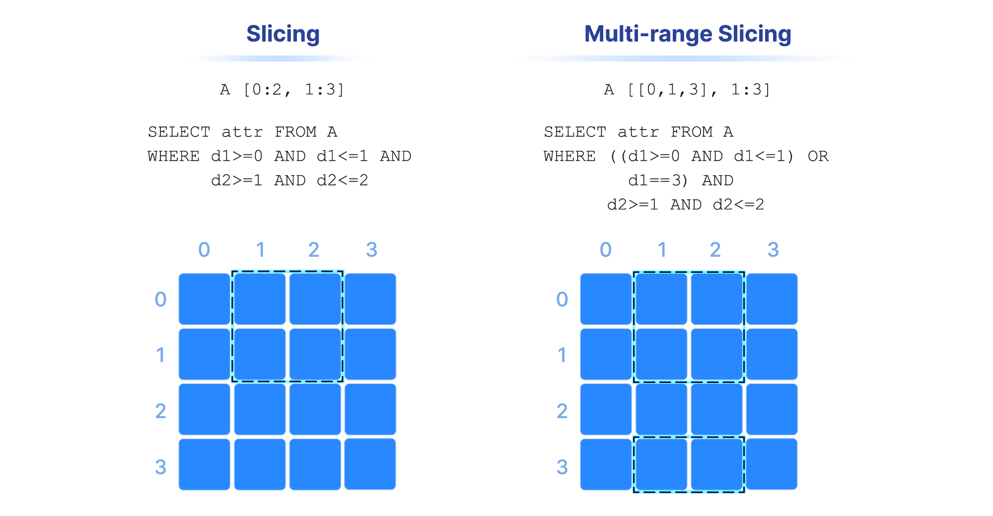
Range conditions on dimensions are often called “slicing” and the results constitute a “slice” or “subarray”. Some examples are shown in the figure below. In numpy notation, A[0:2, 1:3] is a slice that consists of the values of cells with coordinates 0 and 1 on the first dimension, and coordinates 1 , and 2 on the second dimension (assuming a single attribute). Alternatively, this can be written in SQL as SELECT attr FROM A WHERE d1>=0 AND d1<=1 AND d2>=1 AND d2<=2 , where attr is an attribute and d1 and d2 the two dimensions of array A. Note also that slicing may contain more than one range per dimension (a multi-range slice/subarray).

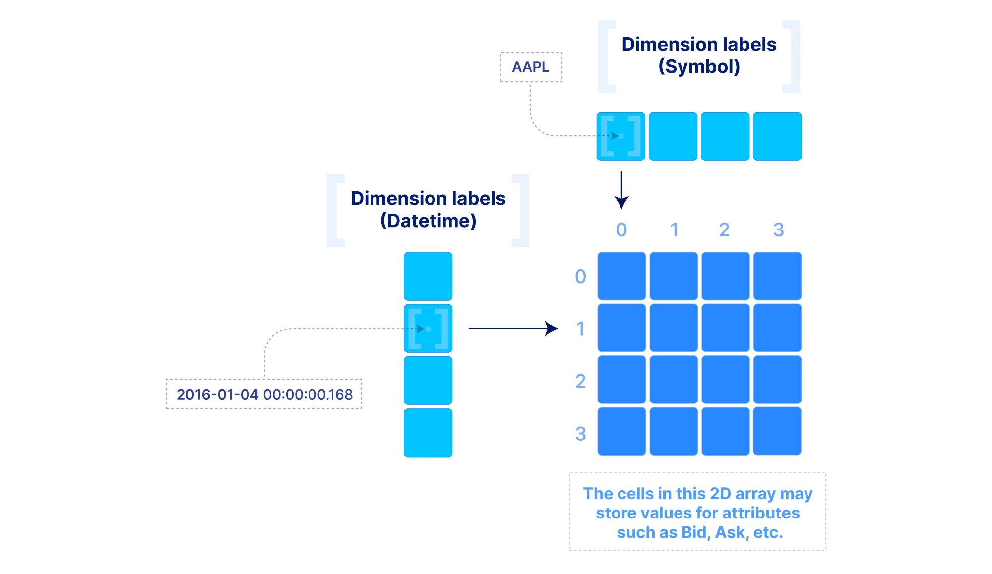
The above model can be extended to include “dimension labels”. This extension can be applied to both dense and sparse arrays, but labels are particularly useful in dense arrays. Briefly stated, a dimension can accept a label vector which maps values of arbitrary data types to integer dimension coordinates. An example is demonstrated below. This is very powerful in applications where the data is quite dense (i.e., there are not too many empty cells), but the dimension fields are not integers or do not appear contiguously in the integer domain. In such cases, multi-dimensional slicing is performed by first efficiently looking up the integer coordinates in the label vectors, and then applying the slicing as explained above. The reason why this may be preferable to simply modeling the data with a sparse array will become clear in the performance section below.

Use cases captured by multi-dimensional arrays

Multi-dimensional arrays have been around for a long time. However, there have been two misconceptions about arrays:

1. Arrays are used solely in scientific applications. This is mainly due to their massive use in Python, Matlab, R, machine learning and other scientific applications. There is absolutely nothing wrong with arrays capturing scientific use cases. On the contrary, such applications are important and challenging, and there is no relational database that can efficiently accommodate them (the reason will become clear soon).
2. Arrays are only dense. Most array systems (i.e., storage engines or databases) built before TileDB focused solely on dense arrays. Despite their suitability for a wide spectrum of use cases, dense arrays are inadequate for sparse problems, such as genomics, LiDAR and tables. Sparse arrays have been ignored and, therefore, no array system was able to claim universality.

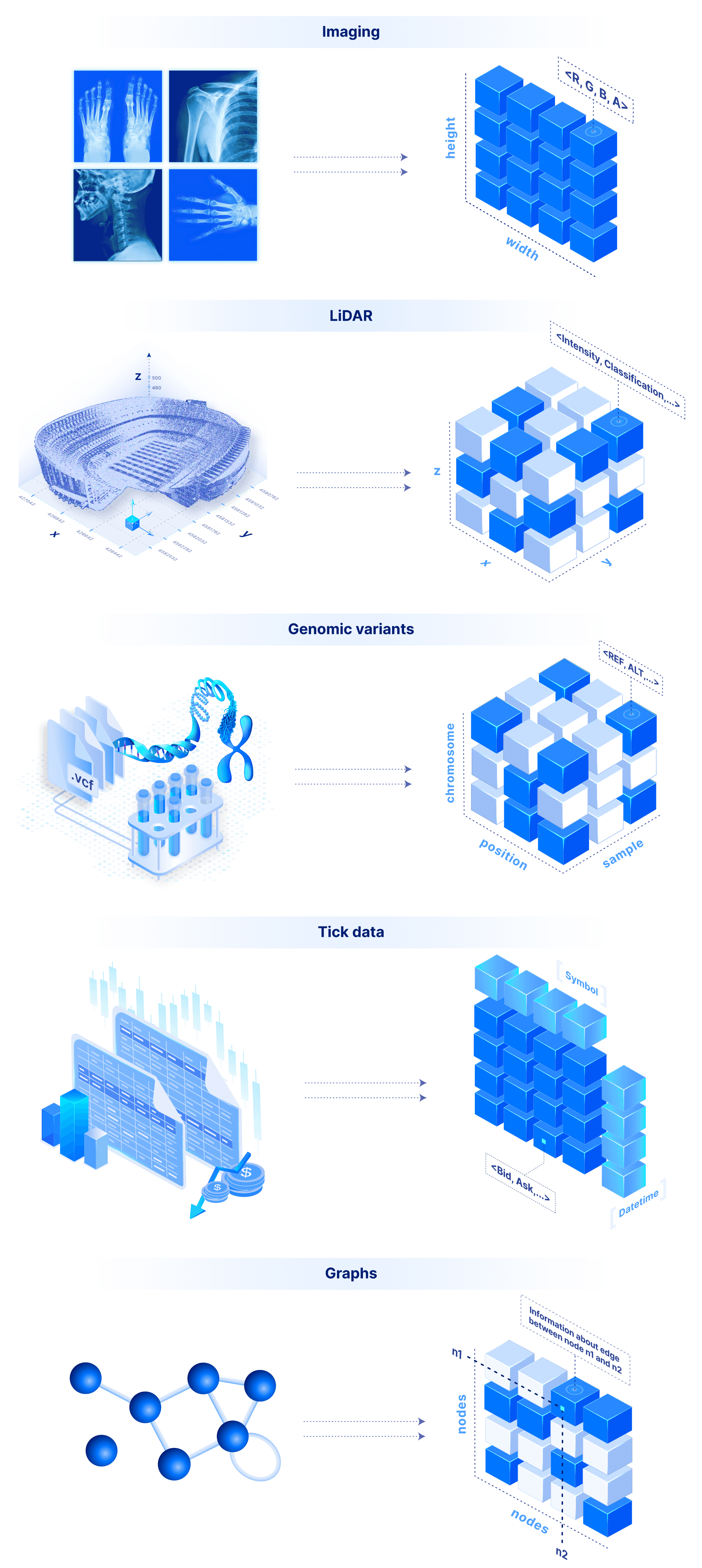
The sky is the limit in terms of applicability for a system that supports both dense and sparse arrays. An image is a 2D dense array, where each cell is a pixel that can store the RGBA color values. Similarly a video is a 3D dense array, two dimensions for the frame images and a third one for the time. LiDAR is a 3D sparse array with float coordinates. Genomic variants can be modeled by a 3D array where the dimensions are the sample name (string), the chromosome (string) and the position (integer). Time series tick data can be modeled by a 2D array, with time and tick symbol as labeled dimensions (this can of course be extended arbitrarily to a ND dense or sparse array). Similarly, weather data can be modeled with a 2D dense array with float labels (the lat/lon real coordinates). Graphs can be modeled as (sparse 2D) adjacency matrices. Finally, a flat file can be stored as a simple 1D dense array where each cell stores a byte.

But what about tabular data? Arrays have a lot of flexibility here. In the most contrived scenario, we can store a table as a set of 1D arrays, one per column (similar to Parquet for those familiar with it). This is useful if we want to slice a range of rows at a time. Alternatively, we can store a table as a ND sparse array, using a subset of columns as the dimensions. That would allow rapid slicing on the dimension columns. Finally, we can use labeled dense arrays as explained above for the time series tick data.

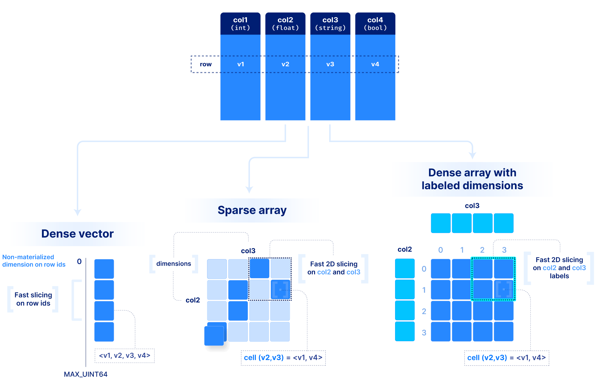
You may wonder how we can make all these decisions about dimensions vs. attributes and dense vs. sparse for each application. To answer that, we need to understand how dense and sparse arrays lay data out on the storage medium, and what factors affect performance when slicing, which is the focus of the next section.

Why arrays are performant for data management

The first step for performance in a system built on the above array model is figuring out the on-disk format. That will dictate the IO cost which is often dominant for a lot of query workloads. I will first explain some of the architectural decisions we took in TileDB Embedded to build an efficient array format. I will then explain how such a format leads to highly efficient slicing operations and summarize all performance factors.

The on-disk format

Let’s start with how we store the dimension coordinate and attribute values.In order to efficiently support cloud object stores and versioned writes, we have chosen a multi-file format, where the values along each dimension or attribute are stored in a separate file. A dense array does not materialize the dimension coordinates, whereas a sparse array must. The figure below shows a dense and a sparse array example. Observe that each cell value across all dimensions and attributes appears in the same absolute position across the corresponding files. Moreover, in variable-length attributes or dimensions, a separate file is needed to store the byte offset of where each value starts in the value file.

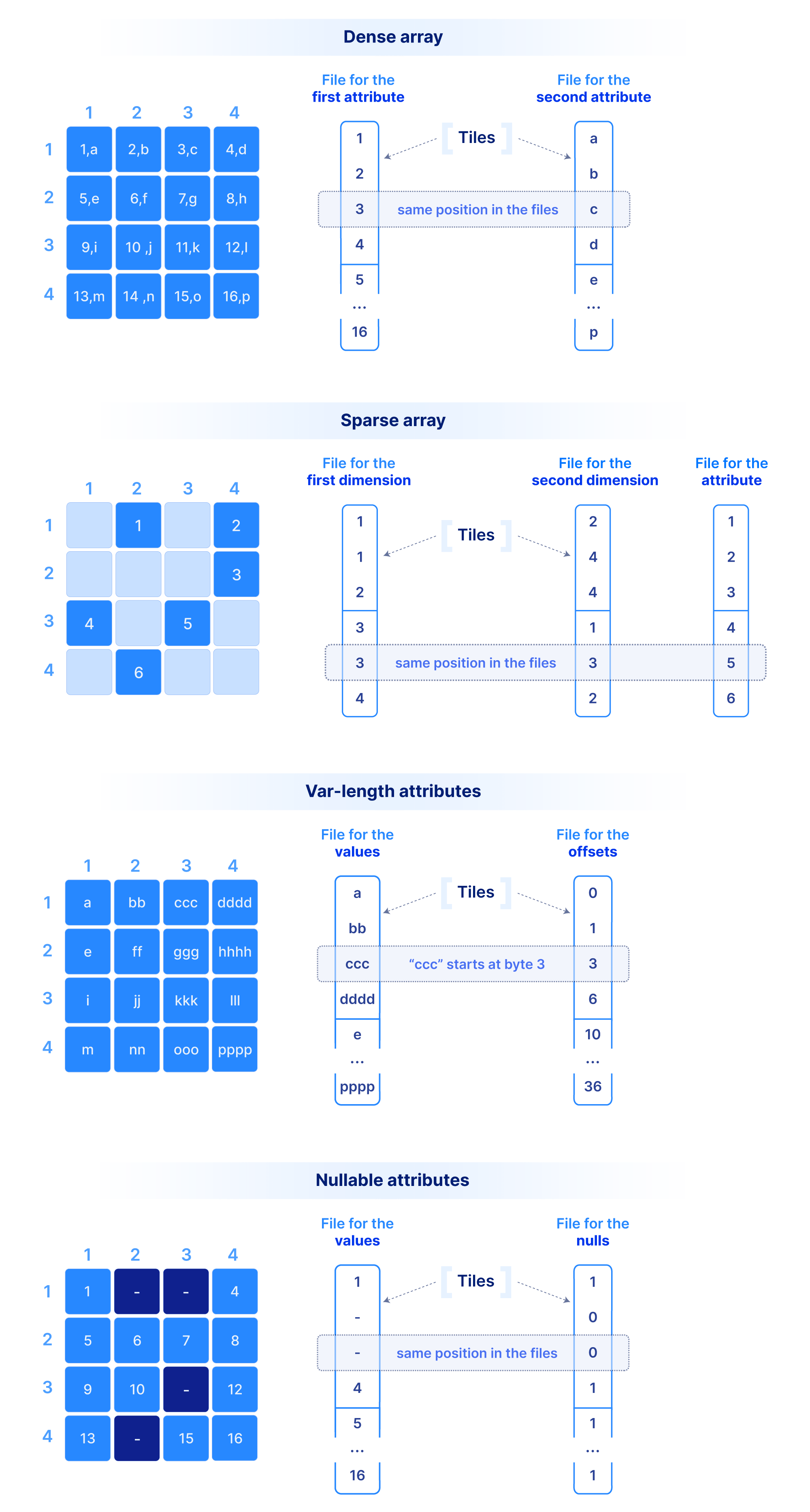
This layout where values of the same type are grouped together is ideal for compression, vectorization and subsetting on attributes/dimensions during queries (similar to other columnar databases). Since typical queries slice subsets of these values, we do not compress the whole file as a single blob. Instead, we tile (i.e., chunk) it into smaller blocks. Therefore, we need a mechanism to create groups of cells. The cells in each tile will appear as contiguous in the corresponding files as shown in the figure above. A tile is the atomic unit of IO and compression, (as well as other potential filters, such as encryption, checksum, etc.).

A question arises: how do we sort the values from a multi-dimensional space, inside the files that are single-dimensional. This order will dictate the position of each cell within its corresponding tile, and the position of the tiles in the file. We call this order the global order of the cells in the array. I will explain the global order and tiling for dense and sparse arrays separately.

In a dense array, the global order and tiling is determined by 3 parameters:

1. The space tile extent per dimension.
2. The cell order inside each tile
3. The tile order

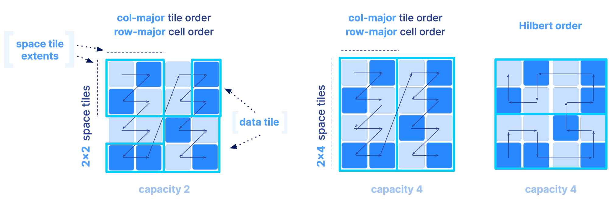
The figure below depicts three different orders as we vary the above parameters. Observe that the shape and size of each tile is dictated solely by the space tile extents.

The sparse array case is slightly different, since tiling only based on space tiles may lead to highly imbalanced numbers of non-empty cells in each tile, which can further impact compressibility and slicing performance. In sparse arrays, the global order could be determined as follows:

1. By specifying the same three parameters as in the dense case, or
2. By using a Hilbert space-filling curve

Once the global order is determined, the tiling is specified by an extra parameter, called the tile capacity, i.e., the number of non-empty cells in each tile. The figure below depicts different global orders for a different choice of all the above mentioned parameters for sparse arrays (a non-empty cell is depicted in dark blue).

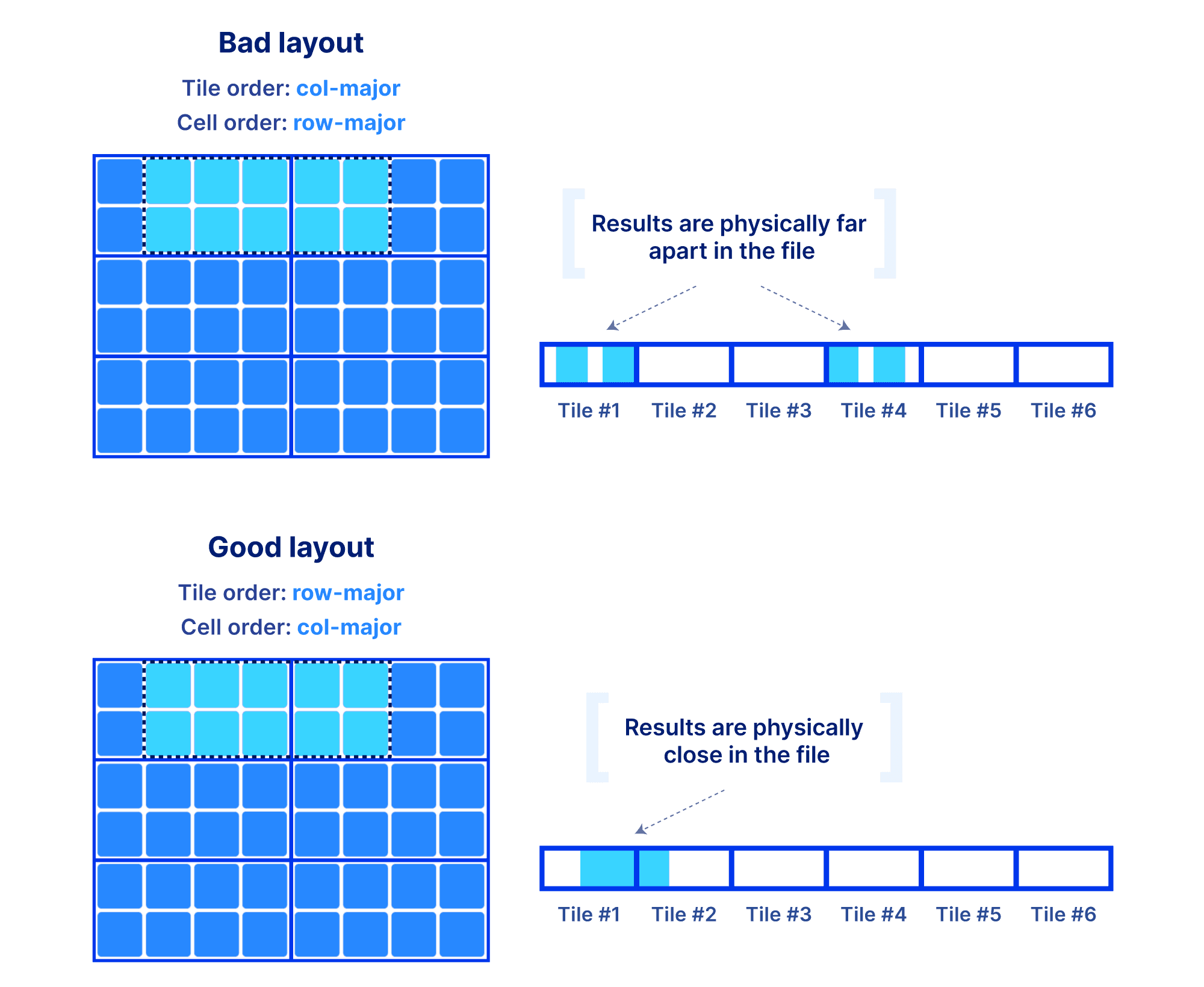
Why is the global order and tiling such a big deal? The global order should retain as much as possible the co-locality of your query results, for the majority of your typical slicing shapes. Remember, the array is multi-dimensional, whereas the file storing the array data is single-dimensional. You have a single chance (unless you want to pay for redundancy) to sort your data in a single 1D order. And that order absolutely dictates the performance of your multi-dimensional queries. The reason is that the closer your results appear in the file, the faster the IO operations to retrieve them. Also the size of the tile can affect performance, since integral tiles will be fetched from storage to memory. The examples below demonstrate some good and bad global orders and tilings for a given slice, focusing on a dense array (similar arguments can be made for the sparse case).

Being perceptive you will say, “I need to know the shape of my slices in order to choose the global order”. In a lot of the applications we have been working on, the typical query patterns are indeed known. If not, arrays still give you the opportunity to define an order that leads to acceptable performance for most of your query patterns. The most important take away here is that arrays provide you with easy and flexible means to manipulate the on-disk representation of your data in order to achieve the desirable performance, for all types of data and applications. And that’s the reason why arrays are universal!

Indexing and accessing array data

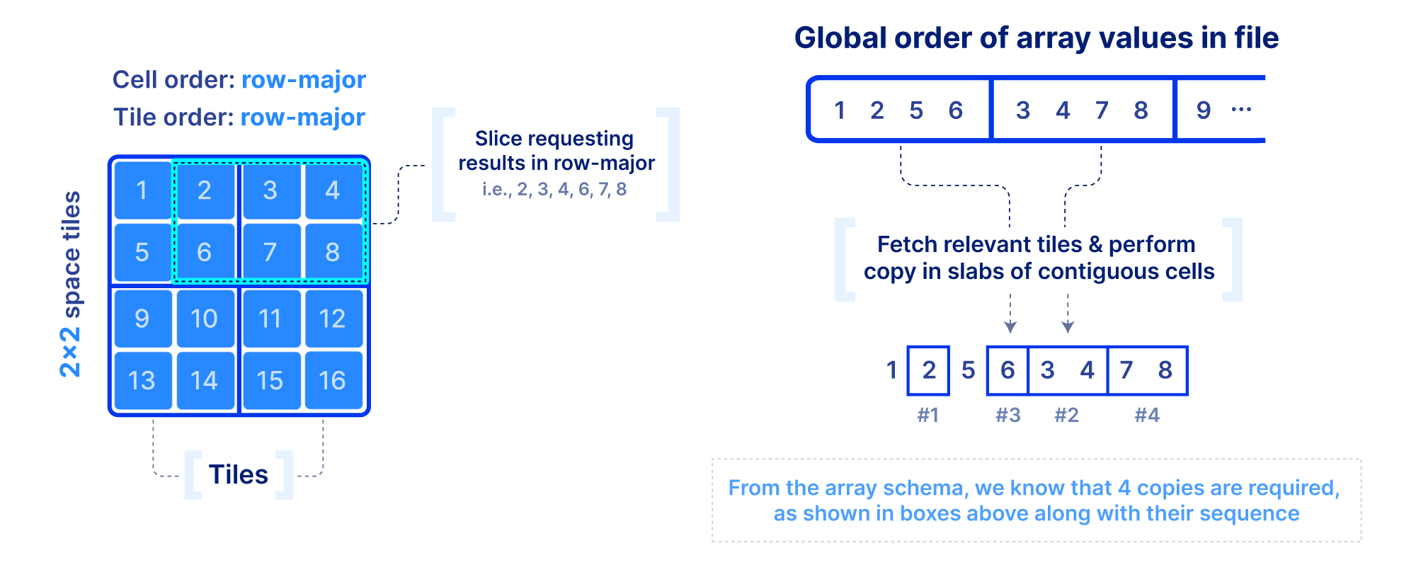
Now that we figured out the on-disk format, how do we efficiently slice an array and what indices shall we optionally build to facilitate the query? First we focus on a dense array and use the example in the figure below. In addition to the slicing query, we know the following: the number of dimensions, the global order, the tiling, and the fact that there are no empty cells in the array. This information is collectively called the array schema. Using solely the array schema and with simple arithmetic, we can calculate the number, size and location of cell slabs (i.e., sets of contiguous cells on the disk) that comprise the query result, without any additional index. Therefore, we can design an efficient multi-threaded algorithm that can fetch the relevant tiles from disk, decompress, and copy the cell slabs into the result buffers, all in parallel. If the algorithm is developed appropriately and the global order and tiling is selected wisely, slicing dense arrays is truly rapid!

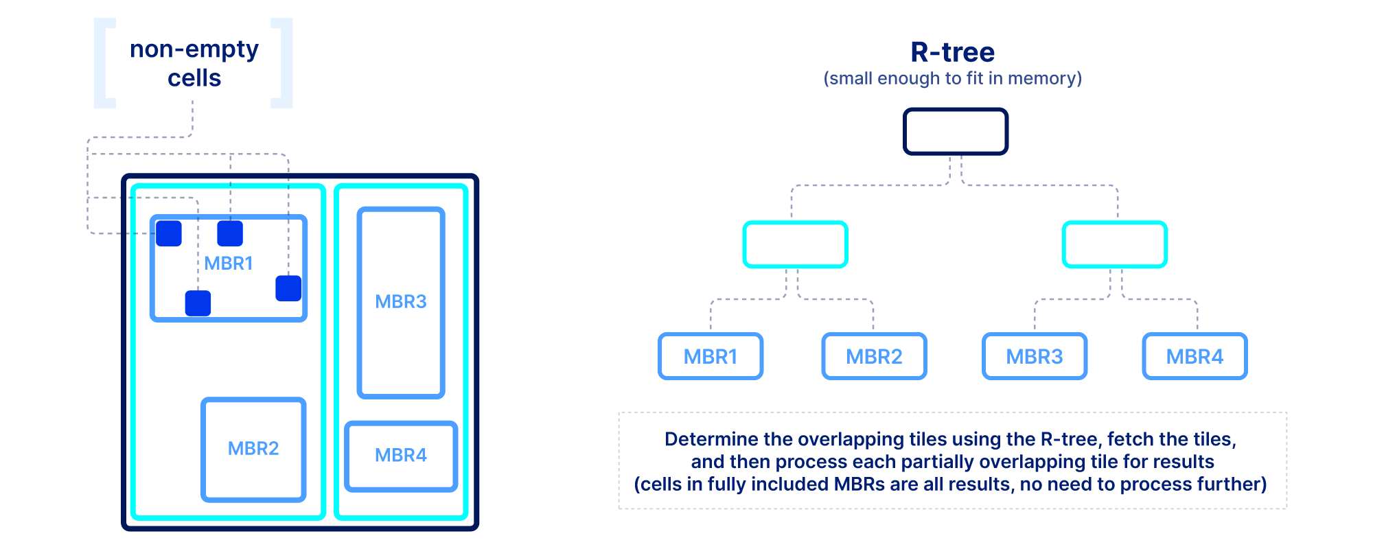
Slicing in sparse arrays is more difficult because we do not know the location of empty cells until the array is written. Therefore, unlike dense arrays, we need to explicitly store the coordinates of the non-empty cells, and build an index on top of them. The index must be small in size so that it can be quickly loaded in main memory when the query is submitted. In TileDB we use an R-tree as an index, but other multi-dimensional indexes exist. The R-tree groups the coordinates of the non-empty cells into minimum bounding rectangles (MBRs), one per tile, and then recursively groups those MBRs into a tree structure. The figure below shows an example. The slicing algorithm then traverses the R-tree to find which tile MBRs overlap the query, fetches in parallel those tiles from storage, and decompresses them. Then for every partially overlapping tile, the algorithm needs to further check the coordinates one by one to determine whether they fall inside the query slice. This simple algorithm, if developed efficiently (using multi-threading and vectorization), can lead to extremely efficient multi-dimensional slicing.

Summary on performance

I already mentioned how some aspects of the array format can affect performance, but below I summarize them all:

1. Dimensions vs. attributes. A data field should be modeled as a dimension if most of the query workloads have a range condition (i.e., slicing) on that field. Otherwise, it should be modeled as an attribute.
2. Number of dimensions. As the number of dimensions increases, you experience diminishing returns. You should select up to 4–5 dimensions that are highly selective for your queries (i.e., have high pruning power). This number is empiric and varies for each application.
3. Global order. The global order determines the locality of the cells with respect to the query and can greatly affect the overall cost.
4. Tile size. If the query slice is too small and the tile is too large, a lot of redundant data is fetched from storage, decompressed, and processed, and therefore the performance degrades. Conversely, if the slice is too large but the tiles too small, extra overhead is incurred for processing numerous tiles.
5. Dense vs. sparse. If all cells in the array must have a value, this array should be dense. If the vast majority of the cells are empty, the array should be sparse. If the array is rather dense, but the dimension coordinates take values from a non-integer domain or are non-contiguous integers, then the array should be dense with labeled dimensions.

As a final remark, it should be clear that arrays can efficiently model tabular data, but not vice versa, which would further justify why relational databases (or tabular formats like Parquet) never found success in the scientific domain. Take for example a simple 2x2 dense array [[1, 2], [3, 4]]. Recall that dense arrays do not materialize the coordinates of the cells, and instead infer where the results are located from the array schema (i.e., dimensionality, global order and tiling). In an array engine, the array values would be serialized as 1, 2, 3, 4 in the file (assuming no tile extents and row-major cell order), and an array would be able to locate value in cell (1, 0), i.e., second row, first column, easily as 3. However, there is no notion of dimensionality in tabular formats. If a tabular format stored the array values in a column as 1, 2, 3, 4, it would not possess the necessary information that the first two values correspond to the first row, and the second two to the second row for this example. Therefore, there would be no way to locate the value of cell (1, 0), unless we created two extra columns explicitly storing the coordinates of every value and scan the table, which would incur significant unnecessary costs. If you find this example trivial, try to imagine how complex it gets in the presence of multiple dimensions, tiling and different tile and cell orders.

Build storage engines, not formats

So far we have designed a great data model and an associated on-disk format that could lead to excellent performance, but where do we go from here? Before answering that, I will point out a few pitfalls that we observed with other array systems:

• Focus on dense arrays. Three other great array systems we know of, SciDB, HDF5 and Zarr, focused solely on dense arrays. As mentioned above, dense arrays have a wide range of applications, but cannot support use cases with sparse data, such as LiDAR, genomics, tables and more.
• Built for a single language. For example, Zarr was built in Python and thus it cannot be used from other languages. This limits its usability. Other Zarr implementations are emerging, but the engineering cost to get to parity is extremely high.
• Built for limited backends. For example, HDF5 was built around the idea of a single-file format. That was a good choice for HPC environments and distributed filesystems like Lustre, but it does not work on cloud object stores where all files/objects are immutable. Also object stores pose other constraints around latency that need to be considered in the read algorithm for efficient IO.
• Focus on the format spec. There is nothing wrong about defining and disclosing the array format spec. The largest problem with format specs is that the implementation burden is left to the higher level applications (e.g., SQL engines like MariaDB, or computational frameworks such as Spark). This in turn poses two issues: (1) there is a lot of reinvention of the wheel around building the storage layer that will parse and process the format, and (2) different communities need to agree on evolving the format spec, since changing it will lead to all applications using it to break.

I argue that the data model and a format spec are not sufficient. We need to focus on building a powerful storage engine to support and evolve the array data model and format, with the following design principles (which we followed in TileDB Embedded):

• Support for both dense and sparse arrays, so that we can achieve universality.
• Built in C++ for performance, but wrapped in numerous APIs (C, C++, C#, Python, R, Java, Go, Javascript) for wider adoption. These APIs can also facilitate the integration with SQL engines, computational frameworks, machine learning libraries and other domain-specific tooling.
• Optimized for all backends (POSIX-based, HDFS, S3, GCS, Azure Blob Storage, MinIO, even RAM), by abstracting the IO layer within the storage engine and making it extendible.
• Focus on the storage engine, not the format spec. Higher level applications should be integrating with the storage engine and use its APIs. They should be completely oblivious to the underlying format spec. This will allow the storage engine to swiftly evolve and improve the format, without the higher level applications breaking.

The above are only the “basic” functionalities a storage engine should have. In order to build the foundation for a universal database, some more advanced features are needed:

• Versioning and time traveling, which are vital for any database system.
• Computation push-down, such as conditions on attributes and more complex queries such as group-by aggregations. This can eliminate unnecessary data copying and movement.

The main takeaway is that multi-dimensional arrays can be powerful if supported by the right storage engine. And building a carefully engineered array engine is quite the undertaking. Fortunately, today there exists such an engine, called TileDB Embedded, and it is open-source under the MIT license. It is my hope that its design principles will motivate new array engines to emerge.

Conclusion

In this blog post I made the case that multi-dimensional arrays are a powerful data model that can serve as the foundation of a universal database that can capture all data types and applications. I explained the benefits of universality and presented the array data model. Then I described an efficient on-disk array format and elaborated on why it can lead to excellent performance via a technical deep dive. Finally, I argued that the array model and on-disk format are not sufficient without building a powerful storage engine to support and evolve them.

I am always looking forward to community feedback. You can find me and my team in the TileDB Slack workspace and forum, or you can contact us directly. For further reading, I suggest the TileDB docs and the following blogs / webinars:

• Debunking “Purpose-Built Data Systems”: Enter the Universal Database
• A deep dive into the TileDB data format & storage engine
• Technical walk-through of the TileDB Cloud universal database

A huge thanks to the entire TileDB team for making this possible!