TileDB is a powerful multimodal database, which allows you to manage and analyze complex data faster, while dramatically simplifying your data infrastructure. TileDB can handle a vast range of use cases with complex data, including genomics, point clouds, biomedical and satellite images, vector embeddings, dataframes, and many more. But how is it possible that a single database system can efficiently handle so many data modalities in a unified way? The answer lies in a magical data structure, the multi-dimensional array, which is a first class citizen in TileDB.

All use cases and integrations in the TileDB world use arrays behind the scenes. Understanding the basics of manually creating TileDB arrays will help you on your journey to becoming a TileDB power user, such that you can either understand and optimize the vertical solutions based on TileDB, or for creating your next amazing product offering on top of TileDB. In this introductory article, I will show you how to create and use two important variations of arrays (dense and sparse), and attach useful array metadata.

All the code included in this article can run locally on your machine using the Python wrapper of the open-source TileDB library (conda install -c conda-forge tiledb-py pyarrow pandas), but we will also include notebooks that you can run directly on TileDB Cloud (sign up and we’ll give you free credits).

Dense vs. Sparse and Dimensions vs. Attributes

When creating a new array, among other things that I will explain in future blog posts, you need to make two important decisions:

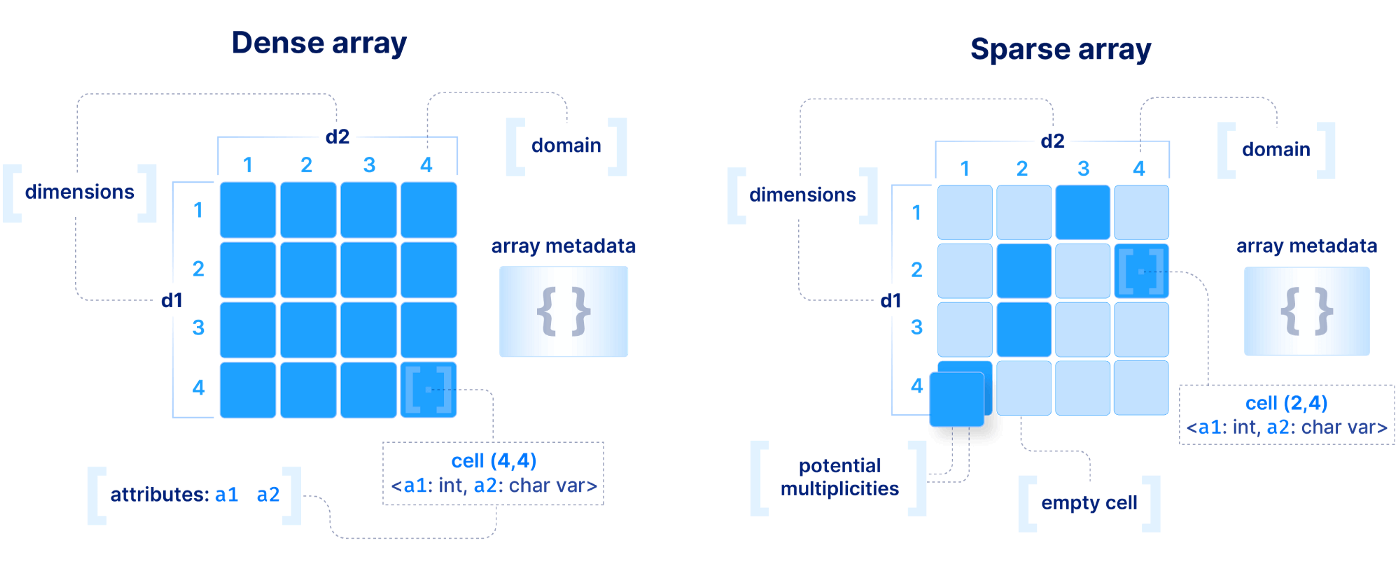
• What is a dimension and what an attribute? The dimensions orient the multi-dimensional space of the array (composed of cells), whereas the attributes specify what kind of values are stored inside each of the cells of the multidimensional space. In a very loose way, think of the dimensions as special attributes of your data where range search can happen very very fast in TileDB. A very simple analogy is an index on a dataframe: the indexed columns are the dimensions, and the rest of the columns are the attributes.
• Dense or sparse? At a very high level, a dense array must have a value in every single one of its cells, even if it is empty. A sparse array may have empty cells that TileDB will never materialize. The decision is heavily dependent on the application. For example, an image is a 2D dense array (since every cell should store the value of a pixel). On the other hand, LiDAR datasets (point clouds) are a 3D sparse array, as we want to store only the scanned points in the vast (infinite) 3D geographical space.

These two decisions need to be specified in what we call the array schema, which describes all the information one needs to understand the basic configuration of an array. Here is a 2D example of a dense and sparse array, just for reference (we will cover a lot more about arrays and their schemas in subsequent articles).

Dense array example

In this example, I will create a 2D dense array with two attributes.

I'll get started by creating the two dimensions:

dd1 = tiledb.Dim(name="d1", domain=(0, 3), tile=2, dtype=np.int32)
dd2 = tiledb.Dim(name="d2", domain=(0, 3), tile=2, dtype=np.int32)

Above, the domain parameter specifies the lower and upper bounds of each Dim object's range; we’ll call it the dimension domain. The type of the dimensions is 32-bit integer. Let’s ignore the tile parameter for now. Collectively, the dimensions define the array domain specified as follows:

ddom = tiledb.Domain(dd1, dd2)

That effectively will create a 4x4 dense array.

Next, I'll create the two attributes, the first will be string and the second 64-bit float:

da1 = tiledb.Attr(name="a1", dtype=np.dtype('U0'))
da2 = tiledb.Attr(name="a2", dtype=np.float64)

With the domain and attributes of the array set, these two pieces come together to create the array's schema:

dschema = tiledb.ArraySchema(domain=ddom, sparse=False, attrs=[da1, da2])

While you can omit sparse=False above — the default behavior is to create a dense TileDB array — I included it here for clarity.

Now you're ready to materialize the 2D dense TileDB array on disk:

array_dense = os.path.expanduser("~/array_dense")
tiledb.Array.create(array_dense, dschema)

I can open the array and inspect its schema:

A = tiledb.open(array_dense)
print(A.schema)

This gives me the following output:

ArraySchema(
  domain=Domain(*[
    Dim(name='d1', domain=(0, 3), tile=2, dtype='int32'),
    Dim(name='d2', domain=(0, 3), tile=2, dtype='int32'),
  ]),
  attrs=[
    Attr(name='a1', dtype='<U0', var=True, nullable=False),
    Attr(name='a2', dtype='float64', var=False, nullable=False),
  ],
  cell_order='row-major',
  tile_order='row-major',
  capacity=10000,
  sparse=False,
)

Let’s write some data to the entire 4x4 array for both attributes. First, I prepare numpy arrays that will hold the attribute values:

# Values to be written for the first attribute
da1_data = np.array([
    ['apple', 'banana', 'cat', 'dog'],
    ['egg', 'frog', 'gas', 'hover'],
    ['icey', 'justice', 'krill', 'lemming'],
    ['munch', 'nothing', 'opal', 'polyester']], dtype='<U0')

# Values to be written for the second attribute
da2_data = np.array([
    [0.0, 0.1, 0.2, 0.3],
    [1.0, 1.1, 1.2, 1.3],
    [2.0, 2.1, 2.2, 2.3],
    [3.0, np.nan, 3.2, 3.3]], dtype=np.float64)

Second, I will open the TileDB array in write mode and provide the above values in an ordered dictionary.

with tiledb.open(array_dense, 'w') as A:
    A[:] = {'a1': da1_data, 'a2': da2_data}
    # For an array with one attribute, write the numpy array directly into TileDB
    # e.g., `A[:] = da1_data`

I can read all of the data back as an ordered dictionary of numpy arrays as follows:

A = tiledb.open(array_dense) # or A = tiledb.open(array_dense, ’r’)
A[:] # Returns an ordered dictionary of 2D numpy arrays

You should get this:

OrderedDict([('a1',
              array([['apple', 'banana', 'cat', 'dog'],
                     ['egg', 'frog', 'gas', 'hover'],
                     ['icey', 'justice', 'krill', 'lemming'],
                     ['munch', 'nothing', 'opal', 'polyester']], dtype=object)),
             ('a2',
              array([[0. , 0.1, 0.2, 0.3],
                     [1. , 1.1, 1.2, 1.3],
                     [2. , 2.1, 2.2, 2.3],
                     [3. , nan, 3.2, 3.3]]))])

TileDB allows you to slice in a variety of ways, without having to bring unnecessary data to main memory from disk.

# Return only subarray [2,2], [1,2]
A[2:3, 1:3] 

OrderedDict([('a1', array([['justice', 'krill']], dtype=object)),
             ('a2', array([[2.1, 2.2]]))])

# Slice only one attribute
A.query(attrs=['a1'])[:]

OrderedDict([('a1',
              array([['apple', 'banana', 'cat', 'dog'],
                     ['egg', 'frog', 'gas', 'hover'],
                     ['icey', 'justice', 'krill', 'lemming'],
                     ['munch', 'nothing', 'opal', 'polyester']], dtype=object))]) 

You can also slice directly in Pandas dataframes, as TileDB arrays can be also logically thought of as dataframes (read the TileDB 101: Dataframes for more).

 # Efficiently slice into Pandas dataframes instead of numpy arrays
A.df[:]

	d1	d2	a1		a2
0	0	0	apple		0.0
1	0	1	banana		0.1
2	0	2	cat		0.2
3	0	3	dog		0.3
4	1	0	egg		1.0
5	1	1	frog		1.1
6	1	2	gas		1.2
7	1	3	hover		1.3
8	2	0	icey		2.0
9	2	1	justice		2.1
10	2	2	krill		2.2
11	2	3	lemming		2.3
12	3	0	munch		3.0
13	3	1	nothing		NaN
14	3	2	opal		3.2
15	3	3	polyester	3.

Sparse array example

I will create a 2D sparse array with one string attribute, reusing many of the previous concepts I explained in dense arrays. I will use a string and a 32-bit float dimension, in order to emphasize that sparse arrays can have heterogeneous dimensions, as well as infinite (!) domains.

To create the array, I will specify the schema similar to the dense case, with the most important difference being sparse=True in the schema creation.

# Create the dimensions
sd1 = tiledb.Dim(name="d1", dtype="ascii")
sd2 = tiledb.Dim(name="d2", domain=(0.0, 10.0), tile=2, dtype=np.float32)

# Create the array domain
sdom = tiledb.Domain(sd1, sd2)

# Create the string attribute
sa1 = tiledb.Attr(name="a1", dtype=np.dtype('U0'))

# Create the array schema
# Setting `sparse=True` indicates a sparse array
sschema = tiledb.ArraySchema(domain=sdom, sparse=True, attrs=[sa1])

# Materialize the array on disk
array_sparse = os.path.expanduser("~/array_sparse")
tiledb.Array.create(array_sparse, sschema)

Let’s inspect the sparse array schema.

B = tiledb.open(array_sparse)
print(B.schema)

This gives the following output:

ArraySchema(
  domain=Domain(*[
    Dim(name='d1', domain=('', ''), tile=None, dtype='|S0', var=True),
    Dim(name='d2', domain=(0.0, 10.0), tile=2.0, dtype='float32'),
  ]),
  attrs=[
    Attr(name='a1', dtype='<U0', var=True, nullable=False),
  ],
  cell_order='row-major',
  tile_order='row-major',
  capacity=10000,
  sparse=True,
  allows_duplicates=False,
)

I'll create new numpy arrays for my dimensions and attributes. Note that with sparse TileDB arrays, I must pass a 1D numpy array for each dimension in order to specify the so-called coordinates of each non-empty cell (since TileDB does not materialize empty cells). There should be a 1-to-1 correspondence between the values passed for each dimension and attribute.

sd1_data = np.array(["a", "bb", "ccc", "dddd", "e", "f", "g", "h", "i", "j", "k", "l", "m", "n", "o", "p"], dtype='<U0')
sd2_data = np.array([0. , 0.01, 0.02, 0.03, 0.04, 0.05, 0.06, 0.07, 0.08, 0.09, 0.10, 0.11, 0.12, 0.13, 0.14, 0.15], dtype=np.float32)
sa1_data = da1_data.flatten() # we’ll simply reuse the dense data

with tiledb.open(array_sparse, 'w') as B:
    B[sd1_data, sd2_data] = sa1_data

The above writes the data into the array on disk. Next let’s read some data from this array.

B = tiledb.open(array_sparse, 'r')
B[:]

OrderedDict([('a1',
              array(['apple', 'banana', 'cat', 'dog', 'egg', 'frog', 'gas', 'hover',
                     'icey', 'justice', 'krill', 'lemming', 'munch', 'nothing', 'opal',
                     'polyester'], dtype=object)),
             ('d1',
              array([b'a', b'bb', b'ccc', b'dddd', b'e', b'f', b'g', b'h', b'i', b'j',
                     b'k', b'l', b'm', b'n', b'o', b'p'], dtype=object)),
             ('d2',
              array([0.  , 0.01, 0.02, 0.03, 0.04, 0.05, 0.06, 0.07, 0.08, 0.09, 0.1 ,
                     0.11, 0.12, 0.13, 0.14, 0.15], dtype=float32))])

# Slice portions of the array
# Use the `multi_index` operator for string dimensions,
# which respects TileDB's inclusive semantics
B.multi_index["c":"g", 0.02:0.06] 

This should produce the following:

OrderedDict([('d1', array([b'ccc', b'dddd', b'e', b'f', b'g'], dtype=object)),
             ('d2', array([0.02, 0.03, 0.04, 0.05, 0.06], dtype=float32)),
             ('a1',
              array(['cat', 'dog', 'egg', 'frog', 'gas'], dtype=object))])

While numpy doesn't support dimensions on data types like strings and floats, TileDB's numpy-like slicing will try its best to make queries work like B["c":"g", 0.02:0.06]; however, it's important to note that this approach could produce unexpected results. For example: B["c":"g", 0.02:0.06] considers inclusive ranges and returns the attribute value "gas" and the dimension values "g" and 0.06, even though I would expect these ranges to be exclusive on the right side, in the spirit of numpy's slicing semantics. For cases like this, TileDB provides a multi_index[] operator, which treats ranges inclusively.

We can also slice directly into Pandas dataframes (read the TileDB 101: Dataframes for more).

B.df[:]

	d1	d2	a1
0	a	0.00	apple
1	bb	0.01	banana
2	ccc	0.02	cat
3	dddd	0.03	dog
4	e	0.04	egg
5	f	0.05	frog
6	g	0.06	gas
7	h	0.07	hover
8	i	0.08	icey
9	j	0.09	justice
10	k	0.10	krill
11	l	0.11	lemming
12	m	0.12	munch
13	n	0.13	nothing
14	o	0.14	opal
15	p	0.15	polyester

# Ranges are inclusive
B.df["i":"m"]

	d1	d2	a1
0	i	0.08	icey
1	j	0.09	justice
2	k	0.10	krill
3	l	0.11	lemming
4	m	0.12	munch

B.df[:, 0.08:0.09]

	d1	d2	a1
0	i	0.08	icey
1	j	0.09	justice

# Returns empty dataframe
B.df["q":"z", 5.0:8.2]

	d1	d2	a1

With sparse TileDB arrays, it's possible — and often, desirable — to query for ranges within the array's domain but have no data associated with those positions, not even filler values. In the example above, B.df["q":"z", 5.0:8.2] returns an empty pandas dataframe. Go ahead and try B.multi_index["q":"z", 5.0:8.2]. You should get an ordered dictionary of empty 1D numpy arrays. This exact behavior is what makes TileDB so efficient for analyzing sparse datasets, like genomic variants and point clouds, at large scale.

Array metadata

It's often useful to attach basic key-value metadata to a TileDB array, e.g., to describe more information about the array (e.g., its creator). This metadata is stored alongside the array on disk. TileDB metadata supports strings, integers, floats, and tuples.

with tiledb.Array(array_sparse, "w") as A:
    A.meta["author"] = "Broberg"
    A.meta["series"] = 101
    A.meta["version"] = 2.2
    A.meta["tuple_int"] = (1,2,3,4)

Reading array metadata back is done as follows:

A =  tiledb.Array(array_sparse)
print(A.meta.keys())

['author', 'series', 'tuple_int', 'version']

print(A.meta["tuple_int"], A.meta["author"])

(1, 2, 3, 4) Broberg

How arrays look on disk

We will cover all TileDB internals in subsequent articles, but it is worth quickly showing how arrays look on disk when you create and write to them. Each array we created above is a directory that looks as follows:

!tree {array_dense}

/home/jovyan/array_dense
├── __commits
│   └── __1684028668784_1684028668784_c14b817bea4844cc8a401a3b051c9bf9_18.wrt
├── __fragment_meta
├── __fragments
│   └── __1684028668784_1684028668784_c14b817bea4844cc8a401a3b051c9bf9_18
│       ├── a0.tdb
│       ├── a0_var.tdb
│       ├── a1.tdb
│       └── __fragment_metadata.tdb
├── __labels
├── __meta
└── __schema
    └── __1684028659435_1684028659435_f0dcef031e59414d8e0a7307b5da0359

8 directories, 6 files

!tree {array_sparse}

/home/jovyan/array_sparse
├── __commits
│   └── __1684030252304_1684030252304_ae8734ef7db34117bb5e7c57175466ab_18.wrt
├── __fragment_meta
├── __fragments
│   └── __1684030252304_1684030252304_ae8734ef7db34117bb5e7c57175466ab_18
│       ├── a0.tdb
│       ├── a0_var.tdb
│       ├── d0.tdb
│       ├── d0_var.tdb
│       ├── d1.tdb
│       └── __fragment_metadata.tdb
├── __labels
├── __meta
│   └── __1684031877186_1684031877186_05daf8d4e1c14e39a7051f0c7c5da73d
└── __schema
    └── __1684029765034_1684029765034_01c0d0f9d65b480d8e7f759f55a56c48

8 directories, 9 files

In that sense, TileDB follows a multi-file format for its arrays. Soon, you will learn all about the decisions we took to organize the TileDB format in the way shown above.

See you next time

That's it for TileDB 101: Arrays! You can preview, download or even launch the notebook in TileDB Cloud.

We'd love to hear what you think of this article. Join our Slack community, or let us know on Twitter and LinkedIn. Look out for future articles in our 101 series on TileDB. Until next time!