In this introductory 101 article I will cover the basics of how to ingest point cloud data into a TileDB array, and then read and visualize this data in flexible ways.

A point cloud dataset is a collection of non-uniformly distributed points in space, usually in 3 or 4 spatiotemporal dimensions. Point clouds are found in SONAR, LiDAR and surveying applications and are a fundamental data source in digital twin applications. Each point is associated with a set of attributes that describe that point, including its location as X, Y, Z coordinates in the 3D space, and colorization attributes such as Red, Green, and Blue.

In this tutorial I will ingest point cloud data into a sparse TileDB array from a LAZ file, and then read from the array into numpy arrays and pandas dataframes using Python (noting though that TileDB supports numerous language APIs). I will cover querying the data in various ways; in the 3D space, across attribute values and even using SQL. I will also show you how to visualize the point cloud data using the powerful gaming engine BabylonJS originally developed and supported as an open source project by Microsoft.

Setup

The code in this article can be run locally on your own machine using the TileDB open-source library TileDB Embedded and the TileDB Python API. You will also need the Python wrapper of the PDAL library.

It is recommended to activate a fresh conda environment with mamba and install the needed packages:

mamba create -n pointclouds-101 -c conda-forge tiledb-py libtiledb-sql-py pyarrow pandas sqlalchemy pdal python-pdal ipywidgets==7.7.2 jupyterlab==3.4.5

You will also need to install TileDB-PyBablyonJS and its dependencies:

conda activate pointclouds-101
pip install pybabylonjs opencv-python

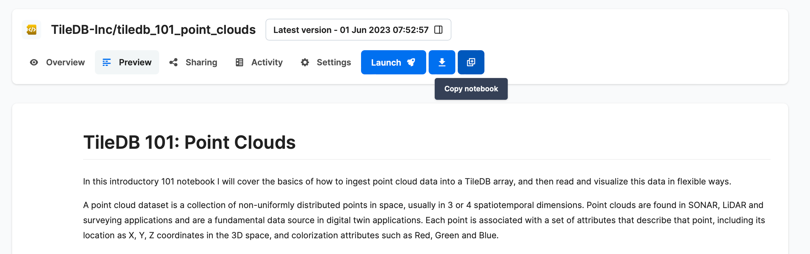
Alternatively, you can run the tutorial notebook in a JupyterLab environment on TileDB Cloud (sign up and you will receive free credits), which comes with all the necessary packages pre-installed. If you’d like to make modifications to the notebook, you can copy the notebook to your account with the Copy button as shown below, then launch a notebook server on TileDB Cloud by clicking the Launch button from the preview page on your copy of the notebook.

Basic ingestion

Let's start by ingesting a LAZ file with a PDAL pipeline, loading a small test point cloud dataset from its URL.

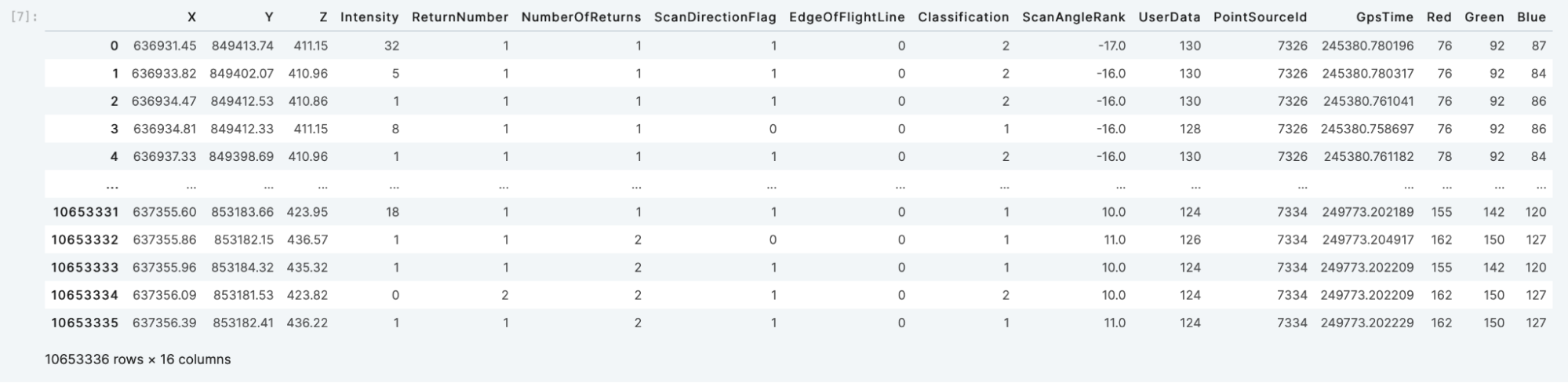
The Python PDAL wrapper fully supports TileDB arrays. It will read the data from the URL and write it out to a TileDB array. This will take a couple of minutes as it is a non-trivial dataset. A successful ingestion will print the number of ingested points (10,653,336 in this example).

# Import the required libraries
import tiledb
import pdal

# The URL of the LAZ file to ingest
data = "https://github.com/PDAL/data/blob/master/workshop/autzen.laz?raw=true"

# The name of the array to write data to
array_name = "pointcloud-101"

# Run the PDAL pipeline - ignore the config details for now
pipeline = pdal.Reader.las(filename=data).pipeline()
pipeline |= pdal.Writer.tiledb(array_name=array_name, x_tile_size=1000, y_tile_size=1000, z_tile_size=100)
pipeline.execute()

I can now print the schema of the newly created array as follows:

A = tiledb.open(array_name)
print(A.schema)

Which gives:

ArraySchema(
  domain=Domain(*[
    Dim(name='X', domain=(-1.7976931348623157e+308, 1.7976931348623157e+308), tile=1000.0, dtype='float64', filters=FilterList([ZstdFilter(level=7), ])),
    Dim(name='Y', domain=(-1.7976931348623157e+308, 1.7976931348623157e+308), tile=1000.0, dtype='float64', filters=FilterList([ZstdFilter(level=7), ])),
    Dim(name='Z', domain=(-1.7976931348623157e+308, 1.7976931348623157e+308), tile=100.0, dtype='float64', filters=FilterList([ZstdFilter(level=7), ])),
  ]),
  attrs=[
    Attr(name='Intensity', dtype='uint16', var=False, nullable=False, filters=FilterList([Bzip2Filter(level=5), ])),
    Attr(name='ReturnNumber', dtype='uint8', var=False, nullable=False, filters=FilterList([ZstdFilter(level=7), ])),
    Attr(name='NumberOfReturns', dtype='uint8', var=False, nullable=False, filters=FilterList([ZstdFilter(level=7), ])),
    Attr(name='ScanDirectionFlag', dtype='uint8', var=False, nullable=False, filters=FilterList([Bzip2Filter(level=5), ])),
    Attr(name='EdgeOfFlightLine', dtype='uint8', var=False, nullable=False, filters=FilterList([Bzip2Filter(level=5), ])),
    Attr(name='Classification', dtype='uint8', var=False, nullable=False, filters=FilterList([GzipFilter(level=9), ])),
    Attr(name='ScanAngleRank', dtype='float32', var=False, nullable=False, filters=FilterList([Bzip2Filter(level=5), ])),
    Attr(name='UserData', dtype='uint8', var=False, nullable=False, filters=FilterList([GzipFilter(level=9), ])),
    Attr(name='PointSourceId', dtype='uint16', var=False, nullable=False, filters=FilterList([Bzip2Filter(level=-1), ])),
    Attr(name='GpsTime', dtype='float64', var=False, nullable=False, filters=FilterList([ZstdFilter(level=7), ])),
    Attr(name='Red', dtype='uint16', var=False, nullable=False, filters=FilterList([ZstdFilter(level=7), ])),
    Attr(name='Green', dtype='uint16', var=False, nullable=False, filters=FilterList([ZstdFilter(level=7), ])),
    Attr(name='Blue', dtype='uint16', var=False, nullable=False, filters=FilterList([ZstdFilter(level=7), ])),
  ],
  cell_order='row-major',
  tile_order='row-major',
  capacity=100000,
  sparse=True,
  allows_duplicates=True,
)

I will not go into detail here, but note that this is a sparse array (sparse=True) and that all compression options are configurable. In future articles, I will cover additional configurations to control compression filters, on-disk layouts, and more.

All data in TileDB are represented as multi-dimensional arrays, and this basic point cloud ingestion created a 3D sparse array with dimension names X, Y and Z. The attributes contain the other variables from the original data. As TileDB is a columnar format (like Parquet), this makes it possible to use point cloud data in unique ways that will speed up your workflows and use new approaches to the data.

The important thing to know at this point is that through the way this array is created, two operations are now very fast:

• Slicing any range across X, Y and Z (e.g., [1:2, 3:4, :])
• Selecting any subset of attributes (e.g., only Red, Green and Blue)

Basic slicing on dimensions

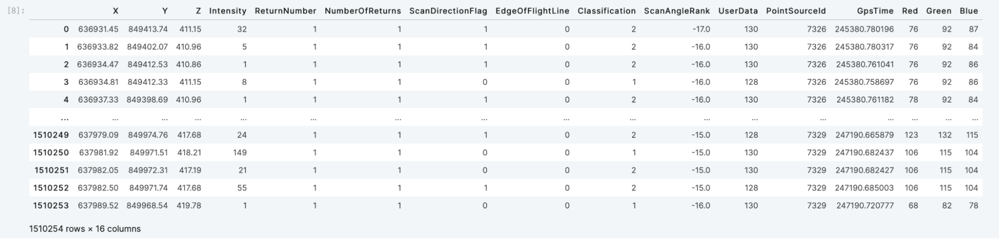
Read all of the data into a pandas dataframe with the TileDB df[] operator:

A.df[:]

You should get the pandas pretty-printed output, with the dimensions X, Y and Z listed on the left:

To slice a subset, simply pass the desired ranges for X, Y and Z in the df operator:

A.df[635600:638000, 849000:850000, :]

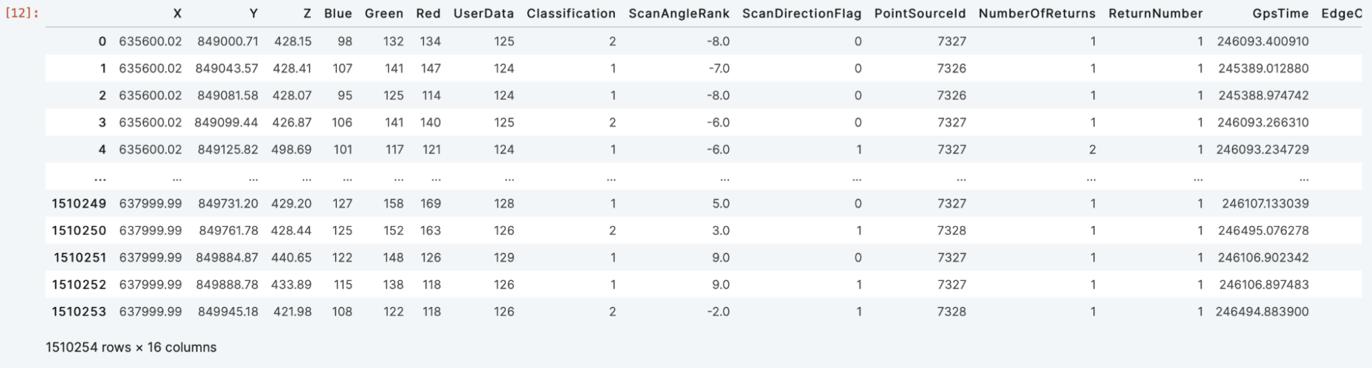
Note how simple this is and now you have point cloud data in a pandas dataframe that you can use in further analysis.

Querying on attributes

In addition to querying on indexed columns (the dimensions), TileDB allows you to subselect attributes and apply filter conditions to them as well. Filtering on attributes may not be as fast as on dimensions; however, TileDB has a lot of internal engineering magic to still make such queries super efficient.

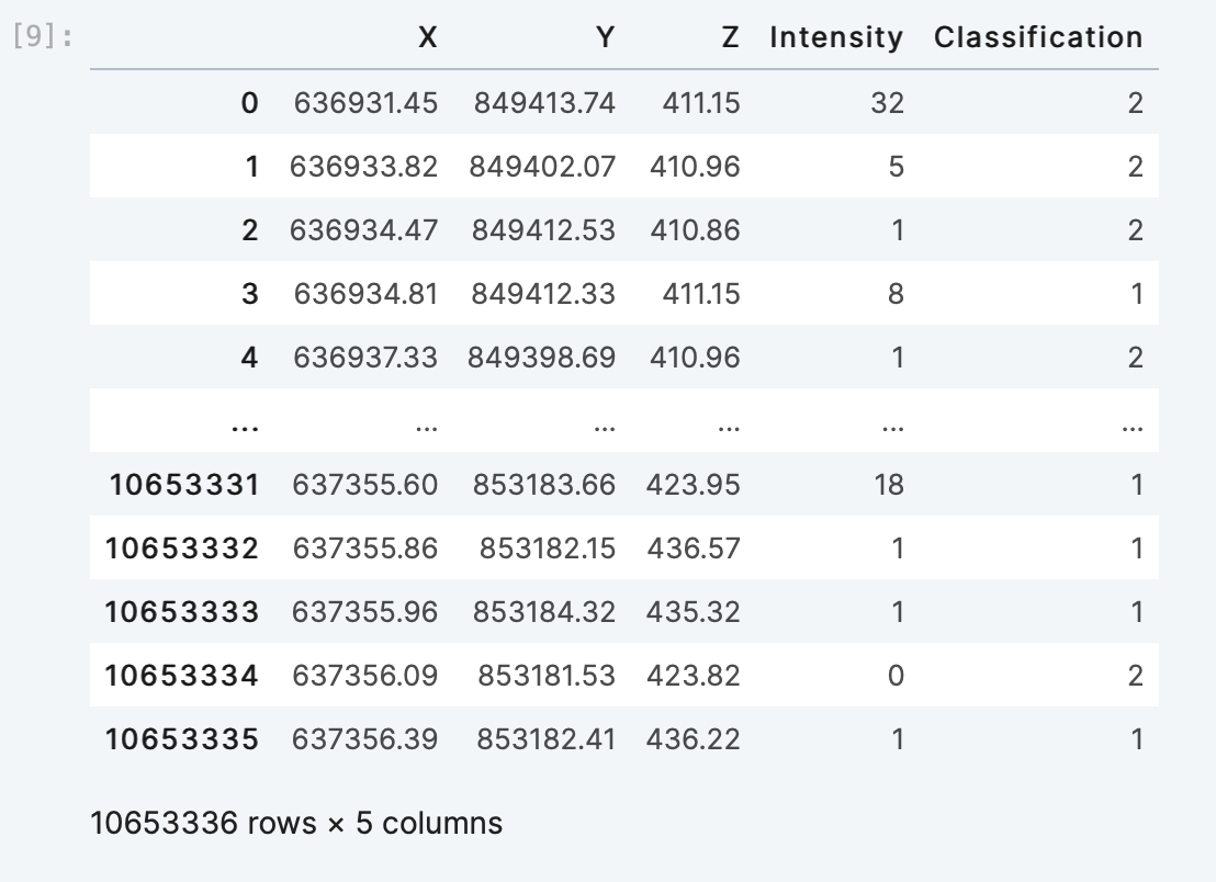
Subselect on the attributes with the query operator:

A.query(attrs=('Intensity', 'Classification')).df[:]

You can also apply a filter condition on attributes as follows:

A.query(cond="Intensity > 10 and Intensity < 100", attrs=['Intensity']).df[:]

Visualizing point cloud data

A visualization is a great way to interact with point cloud data and is one of the most common functionalities of any geospatial workflow. I will keep the description here light, but in future articles I will show you how to configure the display and interactively stream literally billions of points.

I will import pybabylonjs and load the data into a dictionary. Then I will use show.point_cloud() to create the interactive visualization. In the viewer, I will be able to use my mouse to:

• Zoom in and out with the scroll wheel
• Rotate by dragging the mouse with the left button down

from pybabylonjs import Show as show

df = A.query(attrs=('Red', 'Green','Blue')).df[636800:637800, 851000:853000, 406.14:615.26]

data = {
    'X': df['X'],
    'Y': df['Y'],
    'Z': df['Z'],
    'Red': df['Red'],
    'Green': df['Green'],
    'Blue': df['Blue']
}

show.point_cloud(source="dict",
                 data=data,
                 point_size = 4,
                 rgb_max=255,
                 width = 1000,
                 height = 600)

Querying with SQL

TileDB provides an integration with MariaDB for embedded (i.e., serverless) SQL. Follow the installation instructions, and import the following packages:

import tiledb.sql
import pandas as pd

Note: If you get a warning message, you can safely ignore mysql error number 2000; it is an artifact of the way TileDB embeds MariaDB as a library (MariaDB is looking for tables that do not exist since there is no server running).

From here, create a connection object and use pandas's read_sql method. We can write the equivalent SQL to one of our spatial queries above:

db = tiledb.sql.connect()
pd.read_sql(sql=
                f"""
                select * from `{array_name}`
                WHERE X >= 635600 AND X <= 640000 AND
                      Y >= 849000 AND Y <= 850000
                """
                , con=db)

And as expected, we get the same number of results in the SQL query as we do querying the array using the Python API.

It's a best practice to close the array when you're done working with it.

A.close()

See you next time

That's it for TileDB 101: Point Clouds! You can preview, download or launch the notebook from TileDB Cloud.

TileDB is a native fit for massive sparse 3D point clouds and in future tutorials you will learn more about the powerful capabilities of TileDB Embedded and TileDB Cloud for large scale point cloud analysis and visualization.

We'd love to hear what you think of this article. Join our Slack community, or let us know on Twitter and LinkedIn. Look out for future articles in our 101 series on TileDB. Until next time!